Numerical minimisation is at the heart of most electronic structure codes, and are involved in finding the electronic wavefunctions, often the self-consistent charge density, and in relaxing atoms during structural minimisation. Many of these techniques are very sophisticated, and in modern codes they have often been tuned for performance (sometimes heuristically) but there is no guaranteed way to find a global energy minimum, and they will fail. So it is very important to understand how they work, and why they might fail. Monitoring a calculation to ensure convergence is generally worthwhile (though this can easily turn into an unhelpful distraction if taken to extremes).
In general, we assume that the energy can be written in terms of some multi-dimensional vector, \(\mathbf{x}\), which might represent expansion coefficients for the basis functions in the wavefunctions, or the atomic coordinates, or other parameters. We then expand the energy to second order in \(\mathbf{x}\):
\[E(\mathbf{x}) = E_0 - \mathbf{g}\cdot\mathbf{x} + \frac{1}{2}\mathbf{x}^\prime \cdot \mathbf{H} \cdot \mathbf{x}\]where \(\mathbf{g} = -\partial E/\partial \mathbf{x}\) and \(\mathbf{H} = \partial^2 E/\partial \mathbf{x}^\prime \partial \mathbf{x}\), the Hessian, which gives the curvature of the energy surface.
All methods use an iterative approach: we choose a direction in which to optimise, find a minimum along that direction, and repeat until some convergence criterion is reached.
Steepest Descents
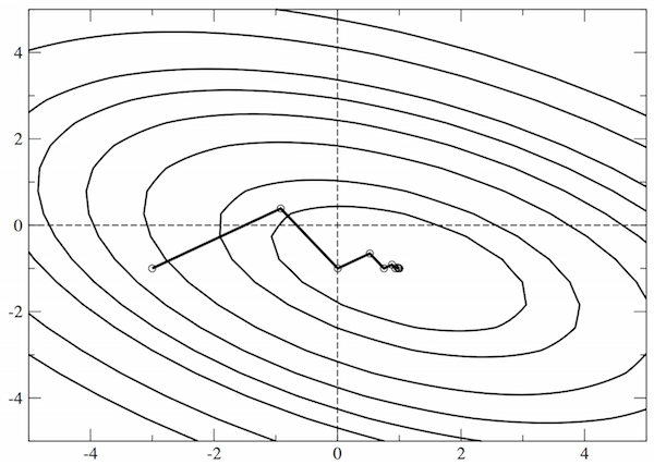
This is the simplest approach to minimisation, which is generally a very poor choice of method. The search direction is always taken as \(\mathbf{g}\), the local downhill gradient. While this is simple, its efficiency depends strongly on the starting point, as illustrated below for a simple, two-dimensional problem where we ought to be able to find the ground state in two steps.
There are two reasons that steepest descents performs so badly: first, it takes no account of previous minimisations; second, it does not use any information about the curvature (the Hessian, above). We can see that the Hessian is useful by taking the equation for \(E\) above, and seeking the stationary points (i.e. solving for \(\partial E/\partial \mathbf{x} = 0\) ):
\[\frac{\partial E}{\partial \mathbf{x}} = -\mathbf{g} + \mathbf{H}\cdot \mathbf{x}\\ \frac{\partial E}{\partial \mathbf{x}} = 0 \Rightarrow \mathbf{g} = \mathbf{H} \cdot \mathbf{x} \Rightarrow \mathbf{x} = \mathbf{H}^{-1}\cdot \mathbf{g}\]If we had the full Hessian, then we could find the minimum, but this would be prohibitively expensive. Improved methods approximate the Hessian, as we will see.
Conjugate gradients
If we choose the search direction, \(\mathbf{h}_n\) at any given iteration \(n\) to be conjugate to the previous search direction, where conjugacy is defined by \(\mathbf{h}_m \cdot \mathbf{H} \cdot \mathbf{h}_n = 0\), then the minimisation of the previous step will not be affected by the present step, and the local curvature is accounted for.
The key to the conjugate gradients method is that this condition can be imposed without calculating the Hessian, if we choose:
\[\mathbf{h}_{n+1} = \mathbf{g}_{n+1} + \gamma \mathbf{h}_n\\ \gamma = \frac{\mathbf{g}_{n+1}\cdot\mathbf{g}_{n+1}}{\mathbf{g}_n\cdot\mathbf{g}_n}\]The maths leading to this formula is not too complex, and can be found in a variety of places[1]. The formula given here is easy to implement, and ensures that successive search directions are conjugate, while successive local gradients are orthogonal. The conjugate gradients method is widely implemented and generally reliable, though requires a good line minimiser (see below for more on this topic) and can fall prey to ill conditioning (also discussed below).
Quasi-Newton methods
The maths for quasi-Newton methods is a little more complex, so I will not detail it here, but the essence of the approach is simple. It generalises the Newton-Raphson approach to multiple dimensions, and builds up an approximation to the inverse Hessian over the course of the optimisation, using the same basic formula for the optimum value of \(\mathbf{x}\) given above. Generally there is a need to truncate the amount of information stored to keep the memory requirements reasonable, but beyond this restriction, the method is very efficient.
Line minimisation
Finding the minimum in a given search direction is a key part of these algorithms. The most robust approach first seeks to bracket the minimum, by taking successively larger steps downhill, and then refines the brackets to find the minimum (using bisection or some more sophisticated approach). The problem with this approach is efficiency: it can require many evaluations, which are computationally wasteful.
A simpler alternative is to take an step with a length that is estimated to be close to the minimum, and use inverse quadratic interpolation to find the minimum from the two points and two gradients available. The approach can work very well when a function is close to quadratic, but often leads to errors in the early stages.
Problems
The most common problem facing numerical optimisation is ill conditioning. If the Hessian has eigenvalues that span a large range, then in some directions the gradient will be very steep, while in others it will be very shallow. This makes it very hard to find the minimum. The ideal solution would be to adjust the curvatures so that they are the same in all directions—which is just the same as inverting the Hessian and applying it to the gradient. Preconditioning approaches estimate an inverse Hessian and use it to improve the convergence of the minimisation. A famous example in electronic structure relates to the kinetic energy of the electrons, and is most easily understood in a plane wave basis set, where the kinetic energy is proportional to \(G^2\) for the wave vector \(\mathbf{G}\). For kinetic energy of large wavevector components dominates the gradient, giving classic ill conditioning; the solution is to scale these components by \(1/G^2\) while leaving the smaller wavevector components unchanged[3]
During structural optimisations, this type of behaviour is often seen when there are very soft modes (where groups of atoms can rotate or rock almost freely). There are other issues: if the electronic minimisation is not fully converged then the structural optimisation can fail (it always pays to check the convergence), and large changes in electronic structure with atomic structure can also give issues (often helped by introducing a larger electronic temperature).
You will inevitably encounter situations where your optimisations or minimisations fail, and understanding how they work can help to diagnose and fix the problem.
[1] While Numerical Recipes is generally the best place to look, I have found the analysis from Jonathan Shewchuk most helpful for this topic[2]
[3] This can be managed using a factor like \(f(G) = G_0^2/(G_0^2 + G^2)\) which is close to 1 if \(G<G_0\) but is close to \(1/G^2\) for large values of \(G\).